Everybody knows the Oktoberfest which takes place in Munich every year. In this blog post series we are going to look into a public available data set and try to gain some insights about the Oktoberfest.
In the first part we load and describe the data. Furthermore, we will analyse the price and consumption of beer and hendl (chicken) over the years.
In the second part we are going to have a closer look at the Bavarian Central Agricultural Festival - also known as “ZLF” - and its influence on beer- and hendl consumption, as well as on visitor count. Further, we are going to look at the influence of the 9/11 terror attacks.
Aim
Since I am currently diving into the field of data analysis and machine learning, I decided to start my first public analysis in order to use the tools I have been learning so far. The aim of this exploratory data analysis was to create some insights about the Oktoberfest using the public available Oktoberfest data set from the Munich Open Data side.
Further, I wanted to explore the Munich Open Data API to export the data from the server.
My biggest aim, though, is to improve my analytic skills by getting feedback from the community.
That is why I would really appreciate your feedback. Feel free to comment on this post and to
contact me.
Methods and Material
For the analysis I used the public available Oktoberfest data set which can be found here. Additional information which can not be found in the data description online, has been provided by the city of Munich via email contact.
Set up Environment
We will start this analysis by loading some required packages:
suppressMessages({
require(httr, quietly = T)
require(tidyverse, quietly = T, warn.conflicts = F)
require(gridExtra, quietly = T, warn.conflicts = F)
require(grid, quietly = T, warn.conflicts = F)
})
Importing Data from API
Having the environment set up, we will use the Munich Open Data API and the httr library to load
our data from the server, and store it as a data.frame within R.
The resource-id (e0f664cf-6dd9-4743-bd2b-81a8b18bd1d2), which we are going to use to get our data
via the API, can be found under additional information (German: “zusätzliche Informationen”) at the
bottom of the data set side.
url <- "https://www.opengov-muenchen.de"
path <- "api/action/datastore_search?resource_id=e0f664cf-6dd9-4743-bd2b-81a8b18bd1d2"

# get raw results
raw.result <- GET(url = url, path = path)

# convert raw results to list
result <- content(raw.result)

# convert results to table
dt <- bind_rows(result$result$records)
Let’s take a quick view at our data to see, if the import went well:
head(dt)## # A tibble: 6 x 9
## hendl_preis jahr besucher_gesamt hendl_konsum dauer bier_konsum
## <chr> <chr> <chr> <chr> <chr> <chr>
## 1 4.77 1985 7.1 629520 16 54541
## 2 3.92 1986 6.7 698137 16 53807
## 3 3.98 1987 6.5 732859 16 51842
## 4 4.19 1988 5.7 720139 16 50951
## 5 4.22 1989 6.2 775674 16 51241
## 6 4.47 1990 6.7 750947 16 54300
## # ... with 3 more variables: bier_preis <chr>, `_id` <int>,
## # besucher_tag <chr>Yes, the API data import worked!
As we see, the columns have German names. We change this for all English speaking readers. By doing so, we also perform some class- and metric corrections.
dt <- dt %>%
  transmute(id = `_id`,
            # class corrections
            year = as.integer(jahr),
            duration = as.integer(dauer),
            hendl_cons = as.integer(hendl_konsum),
            beer_price = as.numeric(bier_preis),
            hendl_price = as.numeric(hendl_preis),
            # class- and additional metric corrections
            beer_cons = as.integer(bier_konsum)*100, # change to L
            visitors_total = as.numeric(besucher_gesamt) * 1000000, # change to nr. of people
            visitors_day = as.integer(besucher_tag)*1000) # change to nr. of people
Data Description
Our data have 9 columns and 34 rows. The data set contains yearly data on beer- and hendl (chicken) consumption from 1985 to 2018. It also provides information about the price of both as well as total visitors, mean daily visitors, and the duration of the Oktoberfest in each year.
The table below gives a quick overview on variable names and their metrics.
| Variable | Metric |
|---|---|
| beer consumption | L |
| beer price | €/Liter |
| hendl consumption | Nr. of Chicken |
| hendl price | €/half chicken |
| total visitors | Nr.of People |
| daily visitors | Nr. of People |
Data Munging
Now we are going to start to get our hands dirty and work with the Oktoberfest data set. We add some information like the years when the Bavarian Central Agricultural Festival (ZLF) took place and other variables which we are going to use either in part 1 or 2 of our analysis.
# generate vector with years in which zlf festival took place
# (every three years up to 1996; every 4 years from 2000 on)
zlf_years <- c(seq(1810,1996, 3), seq(2000, max(dt$year),4))

dt <- dt %>%
  mutate(zlf = factor(ifelse(year %in% zlf_years, 1, 0)),
         hendl_cons_per_visitor = hendl_cons / visitors_total,
         beer_cons_per_visitor = beer_cons / visitors_total) %>%
  select(-id) # remove id column since we don't use it in the analysis
Since there is no missing data in our data set, we can start our analysis.
Data Analysis
In our data analysis we are going to look at the following topics:
Part I:
- Beer price and its consumption
- Hendl price and its consumption
Part II:
- Influence of the ZLF on some variables in our data
- Mean daily visitor count before and after 9/11
We are going to use visualizations and simple modeling techniques to describe the data. Further, we are going to perform statistical tests to compare means in groups.
Beer Price and Consumption
Every year one of the most discussed topics around the Oktoberfest is the increased beer price. People are always complaining that the beer is too expensive. Since we have the historical data on beer prices, our first question on the data set is:
How did the beer price develope from 1985 to 2018?
Modeling Beer Price Development Over the Years
Note: The currency used in the data is €. All prices before the year 2002 have been transformed from DM (German currency before 2002) to Euro.
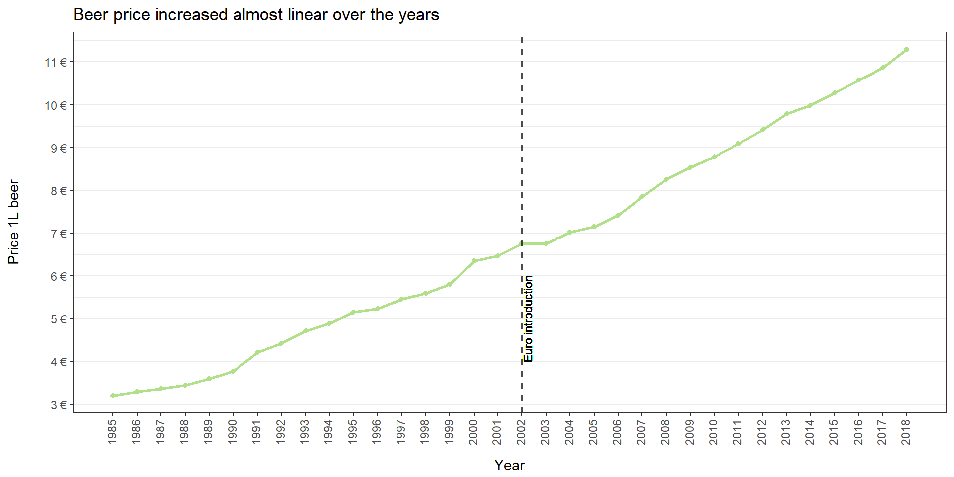
In fact, the price for 1L beer increased almost linear over the years. We will try to use a simple linear regression model to describe the data:
fit_beer <- lm(beer_price ~ year, data = dt)
summary(fit_beer)
##
## Call:
## lm(formula = beer_price ~ year, data = dt)
##
## Residuals:
## Min 1Q Median 3Q Max
## -0.44439 -0.13266 0.00188 0.14010 0.55504
##
## Coefficients:
## Estimate Std. Error t value Pr(>|t|)
## (Intercept) -4.886e+02 8.710e+00 -56.09 <2e-16 ***
## year 2.475e-01 4.352e-03 56.87 <2e-16 ***
## ---
## Signif. codes: 0 '***' 0.001 '**' 0.01 '*' 0.05 '.' 0.1 ' ' 1
##
## Residual standard error: 0.2489 on 32 degrees of freedom
## Multiple R-squared: 0.9902, Adjusted R-squared: 0.9899
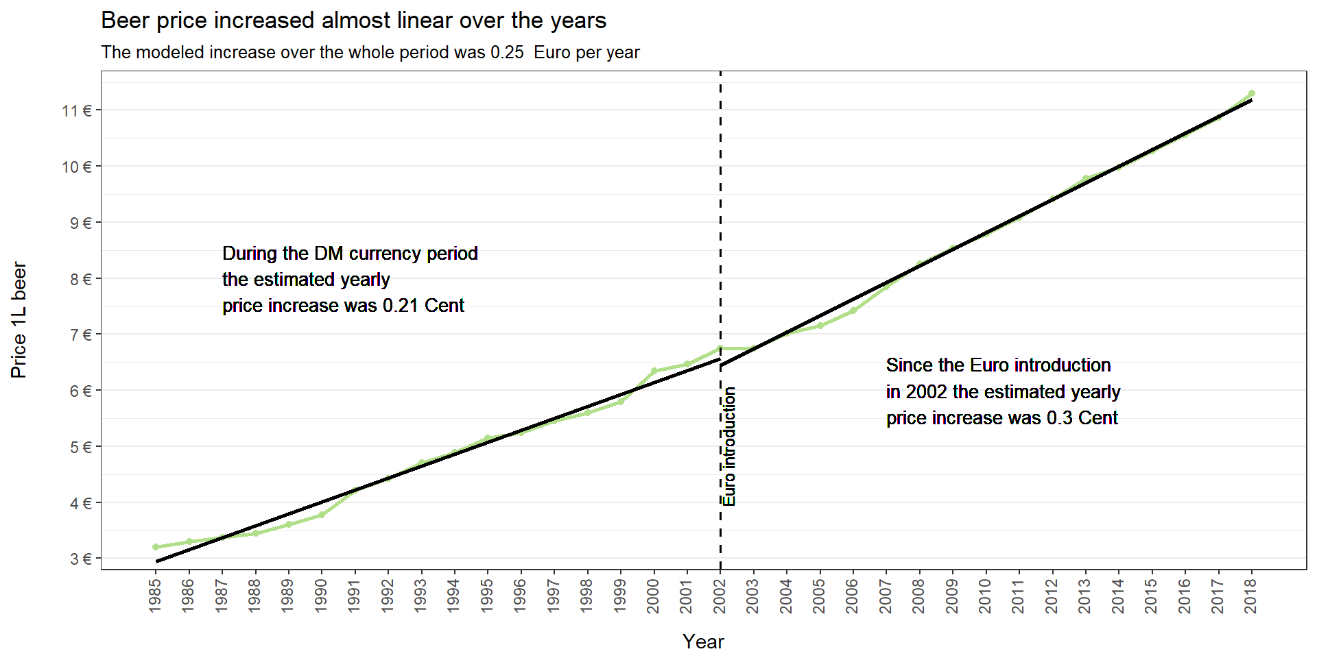
## F-statistic: 3234 on 1 and 32 DF, p-value: < 2.2e-16Our model suggests that the beer price increased by 0.25 Euro per year.
Fitting models to the years with different currencies separately, we see a small difference in estimated price increase per year:
fit_dm <- lm(beer_price ~ year, data = subset(dt, year < 2002))
summary(fit_dm)
##
## Call:
## lm(formula = beer_price ~ year, data = subset(dt, year < 2002))
##
## Residuals:
## Min 1Q Median 3Q Max
## -0.236176 -0.112059 -0.009412 0.077647 0.260000
##
## Coefficients:
## Estimate Std. Error t value Pr(>|t|)
## (Intercept) -4.203e+02 1.399e+01 -30.04 8.17e-15 ***
## year 2.132e-01 7.022e-03 30.37 6.94e-15 ***
## ---
## Signif. codes: 0 '***' 0.001 '**' 0.01 '*' 0.05 '.' 0.1 ' ' 1
##
## Residual standard error: 0.1418 on 15 degrees of freedom
## Multiple R-squared: 0.984, Adjusted R-squared: 0.9829
## F-statistic: 922.2 on 1 and 15 DF, p-value: 6.944e-15fit_euro <- lm(beer_price ~ year, data = subset(dt, year >= 2002))
summary(fit_euro)##
## Call:
## lm(formula = beer_price ~ year, data = subset(dt, year >= 2002))
##
## Residuals:
## Min 1Q Median 3Q Max
## -0.20382 -0.02073 -0.01728 0.01625 0.31294
##
## Coefficients:
## Estimate Std. Error t value Pr(>|t|)
## (Intercept) -5.875e+02 1.148e+01 -51.18 <2e-16 ***
## year 2.967e-01 5.711e-03 51.95 <2e-16 ***
## ---
## Signif. codes: 0 '***' 0.001 '**' 0.01 '*' 0.05 '.' 0.1 ' ' 1
##
## Residual standard error: 0.1154 on 15 degrees of freedom
## Multiple R-squared: 0.9945, Adjusted R-squared: 0.9941
## F-statistic: 2699 on 1 and 15 DF, p-value: < 2.2e-16- In years with DM currency (1985 to 2001) the estimated yearly price increase was around 0.21 Euro per year.
- In the years after the Euro has been introduced (>2001), the estimated yearly price increase was 0.3 Euro per year.
Influence of Beer Price on Consumption
Now that we confirmed that the price increased over the years, the next question which arises is:
Did this increase have a negative influence on mean beer consumption per visitor?
In order to answer this question we are going to start with a visualization of our data:
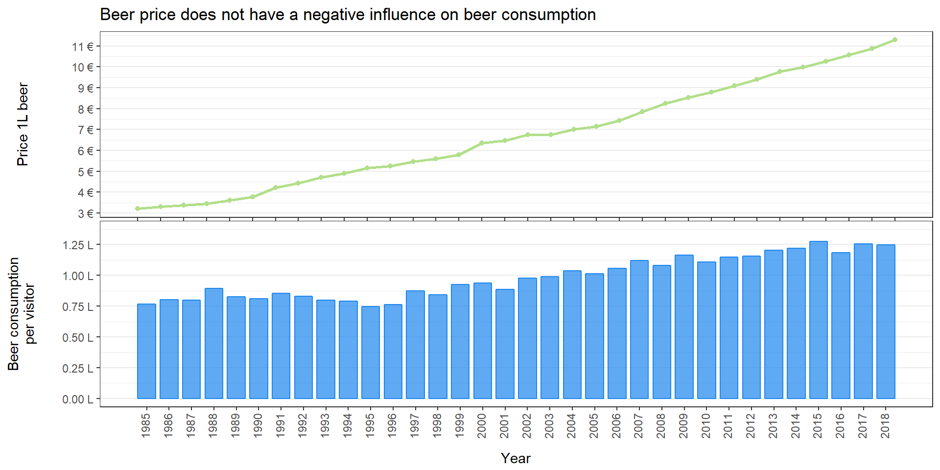
We do not see a decline in mean beer consumption per visitor over the years. In fact, since around year 1999 it seems that it even has been increasing steadily.
To see how the data are correlated we perform a correlation test using the Pearson correlation coefficient:
cor.test(dt$beer_cons_per_visitor, dt$beer_price)##
## Pearson's product-moment correlation
##
## data: dt$beer_cons_per_visitor and dt$beer_price
## t = 17.106, df = 32, p-value < 2.2e-16
## alternative hypothesis: true correlation is not equal to 0
## 95 percent confidence interval:
## 0.9003351 0.9746671
## sample estimates:
## cor
## 0.9494338The test suggests a true correlation with a Pearson correlation coefficient of 0.95. The p-value is way below 0.05 and we have a narrow confidence interval. If we plot the data, all points seem to be around one line:
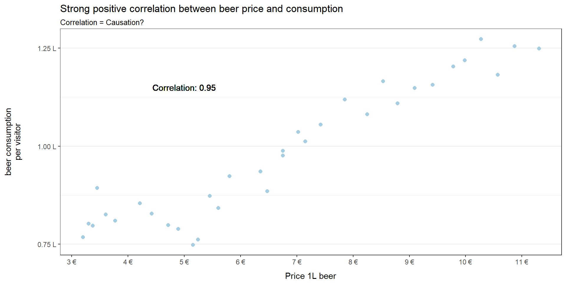
This result would suggest that beer consumption increases the higher the beer price gets. Nevertheless, in my opinion, this is an example that correlation does not imply causation. I think that the increased consumption is a separate phenomena and not caused by increased prices. One reason you can think of might be:
- Oktoberfest gets more and more popular outside of Munich. More and more people from all over the world go there in order to drink a “Maß” beer. For people coming from Australia, Sweden, etc. the beer is still cheap compared to their home. That is why they do not consume less beer with increasing prices since it is still cheap for them.
In conclusion the data set suggests that the price does not seem to have a negative influence on mean beer consumption per visitor.
Hendl Price and Consumption
On the Oktoberfest it is not just about drinking. A lot of people also like to have something to eat besides their beer. So what about the hendl consumption and price development?
Modeling Hendl Price Development
As before we are going to have a look at the price only first:
Important Notes:
- The currency used in the data is €. All prices before the year 2002 have been transformed
from DM (German currency before 2002) to Euro.
- Before the year 2000 the data are mean prices at the selling places. Since 2000 the data are only mean prices inside the tents.
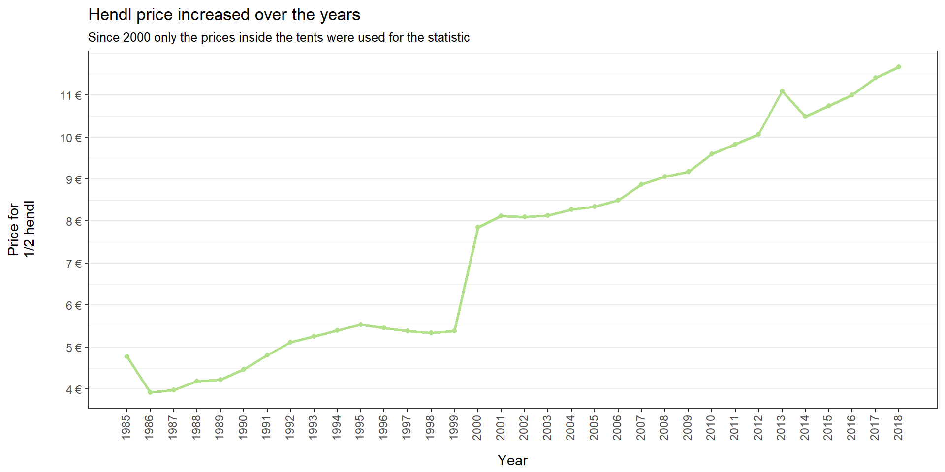
It seems that there was a huge price increase in year 2000. But we need to be careful: As mentioned in the notes above, the data collection method changed in 2000. So we need to compare both periods separately. In the year 2013 we have some kind of price outlier. Here the price was raised a huge amount compared to the steady increase the years before. After that, the price dropped to a level which seems to lie on a line of steady price increase. We will try to model the price increase from year 2000 on using a linear regression model.
fit_hendl <- lm(hendl_price ~ year, data = subset(dt, year >= 2000))
summary(fit_hendl)
##
## Call:
## lm(formula = hendl_price ~ year, data = subset(dt, year >= 2000))
##
## Residuals:
## Min 1Q Median 3Q Max
## -0.33063 -0.14774 -0.08568 0.15142 0.72347
##
## Coefficients:
## Estimate Std. Error t value Pr(>|t|)
## (Intercept) -434.17863 23.20885 -18.71 8.89e-13 ***
## year 0.22084 0.01155 19.12 6.25e-13 ***
## ---
## Signif. codes: 0 '***' 0.001 '**' 0.01 '*' 0.05 '.' 0.1 ' ' 1
##
## Residual standard error: 0.2758 on 17 degrees of freedom
## Multiple R-squared: 0.9555, Adjusted R-squared: 0.9529
## F-statistic: 365.4 on 1 and 17 DF, p-value: 6.254e-13The model suggests that the hendl price increased by 0.22 Euro per year since 2000.
When we add the model to our plot it looks like this:
Influence of Hendl Price on Consumption
Above we saw that the beer price did not have a negative influence on the beer consumption. We are going to ask the same question for the hendl price and consumption. To get a first overview, we plot the data.
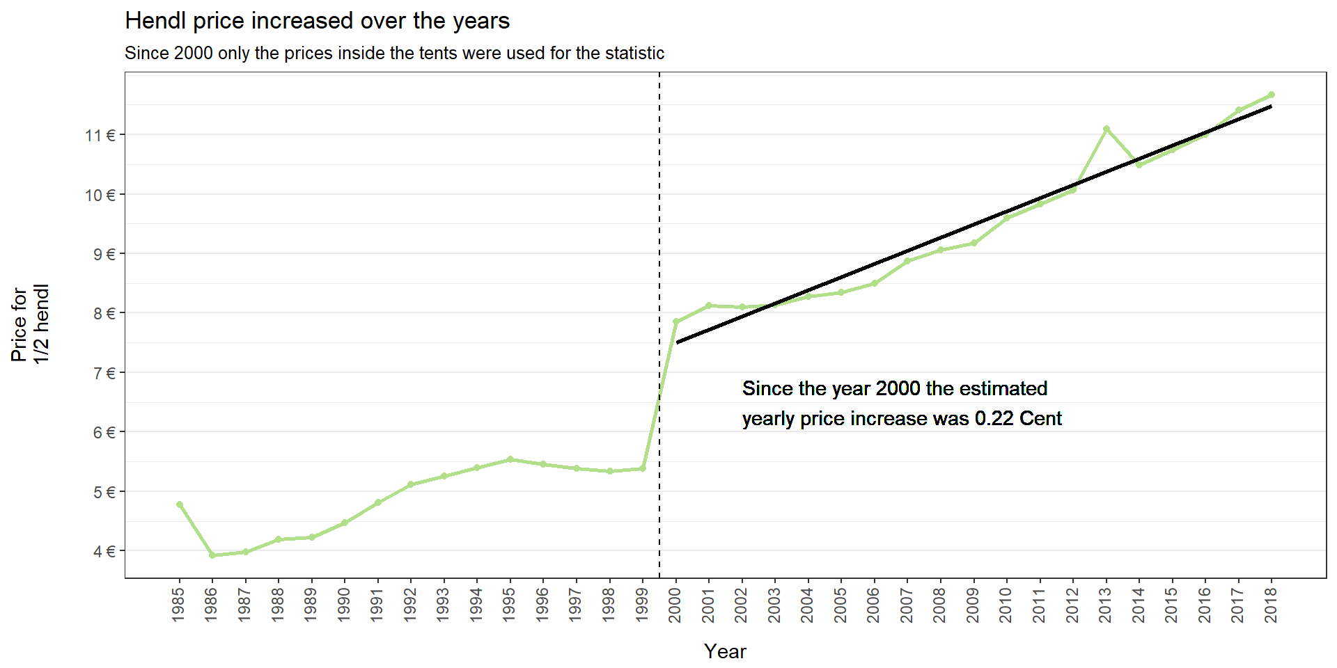
We see that the hendl consumption dropped in 2001 after slowly decreasing from 1991 on.
After the drop, the consumption stayed at a constant level, whereas the price went up.
For me it looks like the hendl consumption being correlated with price until year 2000.
After that the consumption reached a minimum bound. Maybe at this point price sensitivity of the
remaining hendl consumers changes.
We can check the correlation by performing a correlation test using the Pearson correlation coefficient:
with(subset(dt, year < 2000),cor.test(hendl_cons_per_visitor*100, hendl_price))##
## Pearson's product-moment correlation
##
## data: hendl_cons_per_visitor * 100 and hendl_price
## t = -2.1586, df = 13, p-value = 0.05016
## alternative hypothesis: true correlation is not equal to 0
## 95 percent confidence interval:
## -0.812214934 -0.001917789
## sample estimates:
## cor
## -0.513676with(subset(dt, year >= 2000),cor.test(hendl_cons_per_visitor*100, hendl_price))##
## Pearson's product-moment correlation
##
## data: hendl_cons_per_visitor * 100 and hendl_price
## t = -1.4261, df = 17, p-value = 0.1719
## alternative hypothesis: true correlation is not equal to 0
## 95 percent confidence interval:
## -0.6801148 0.1495249
## sample estimates:
## cor
## -0.326885The correlation coefficients suggest a negative correlation for both periods. Nevertheless, the tests confirm the null hypothesis, which says that there is no true correlation between the variables.
For the period before 2000 there is at least a strong tendency
(p = 0.0501576)
for a true negative correlation. Despite that, the confidence interval for the correlation coefficient is very big, which gives us a strong uncertainty.
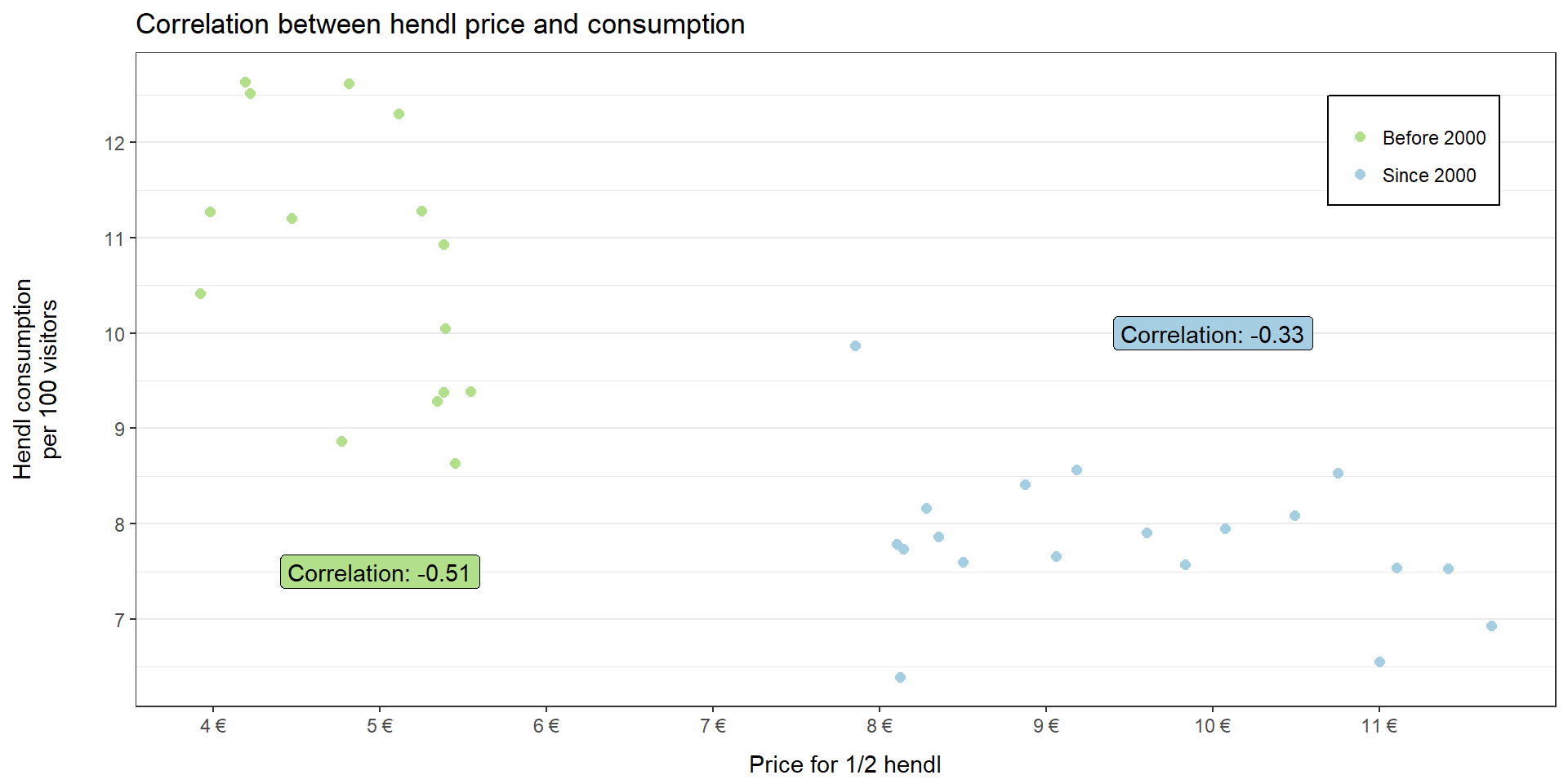
In conclusion we can say that the price seems to have an influence on the hendl consumption up to a specific point. Maybe we could explain the constant level of consumption after reaching that specific price margin with the following hypothesis:
Normally people would buy a hendl up to their specific price boundary. That would mean a steady decrease in consumption with increasing price.
Nevertheless, there are a lot of companies, which rent a table in a tent and invite their employees to come. Most of the time these companies give a free amount of hendl and beer consumption to their employees. I think that a big company’s price sensitivity concerning hendl and beer is not as high as the price sensitivity of a normal Oktoberfest visitor. Thus, even with increasing prices the basic level of consumption does not change a lot.
Conclusion
In the first part of our quick analysis we showed that…
The beer price increased over the years. We modeled a increase of 0.25 Euro per year with differences before and after Euro introduction
The increase in beer price did not have a negative influence on beer consumption. The consumption even went up over the years
Hendl price also increased steadily. For the years since 2000 our model estimated a price increase of 0.22 Euro per year
The hendl price actually seem to have a influence on hendl consumption up to a specific point. We showed a tendency for negative correlation before year 2000.
In addition, I learned that the Munich Open Data API is not that difficult to use.
In the next part of our analysis we will have a closer look on the influence of the ZLF and the 9/11 terror attacks.
Update 2019
Added data from 2018
Acknowledgement
For this part I would like to say thank you to the people who helped me with the ressources for that analysis.I would like to thank Frank Börger and the team from Munich Open Data for answering my questions on the data and providing additional resources. Another great thank you goes to my friend Pat forproofreading.