Everybody knows the Oktoberfest which takes place in Munich every year. In this blog post series we are going to look into a public availabe dataset and try to gain some insights about the Oktoberfest.
In the first part we loaded and described the data. We also analysed the price and consumption of beer and hendl (chicken) over the years.
In this second part we are going to have a closer look at the Bavarian Central Agricultural Festival - also known as “ZLF”. We will look at at its influence on beer and hendl consumption, and on the the visitor count. After that we are going to analyse the influence of the 9/11 terror attacks on mean daily visitor count.
Aim
Since I am currently diving into the field of data analysis and machine learning, I decided to start my first public analysis in order to use the tools I have been learning so far. The aim of this exploratory data analysis was to create some insights about the Oktoberfest using the public available Oktoberfest data set from the Munich Open Data side.
Further, I wanted to try the Munich Open Data API to export the data from the server.
My biggest aim, though, is to improve my analysis skills by getting feedback from the community.
That is why I would really appreciate your feedback. Feel free to comment on this post and to
contact me.
Methods and Material
The data description, as well as the importing and processing steps, can be found in the first part of this series.
Data Analysis - Part II
Bavarian Central Agricultural Festival (ZLF)
The ZLF is an agricultural exhibition which takes place right next to the Oktoberfest at the Theresienwiese. Before 1996 the exhibition was held every three years. From there on it has been taken place every 4 years.
We are going to cover the questions whether or not the ZLF brought more visitors to the Oktoberfest or increased the beer and hendl consumption.
Did the ZLF Bring More Visitor to the Oktoberfest?
Since the ZLF is at the same location as the Oktoberfest a lot of farmers and other visitors who maybe would normally not come to the Oktoberfest are going there in order to see the exhibition. This could have an influence on the mean daily visitor count. We will further investigate this hypothesis by looking at our data. In order to adjust for the duration we will use the mean daily visitor count for our analysis:
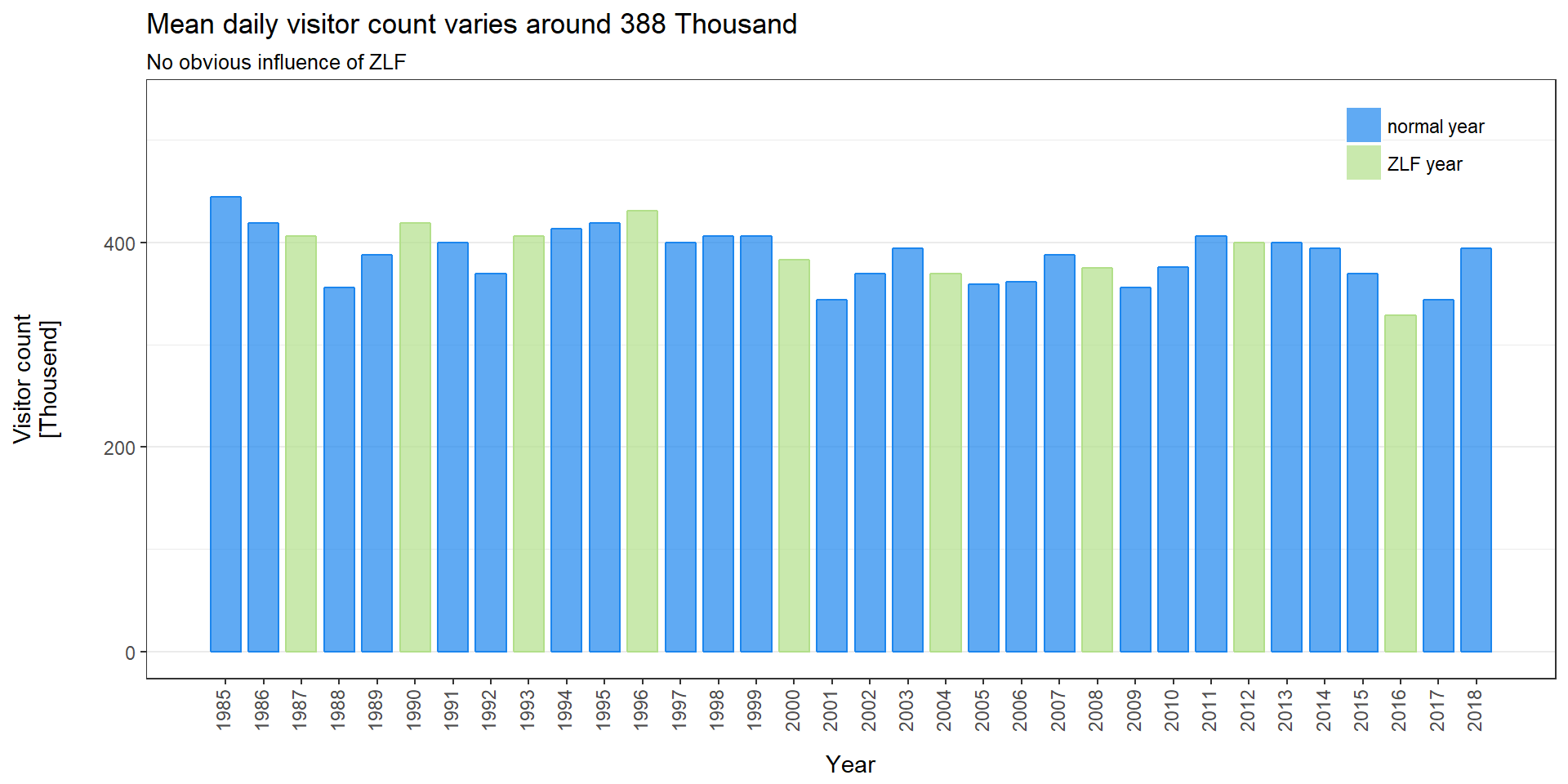
We can see that the mean daily visitor count varies around 388 thousand. There was a huge drop in 2001 which could be due to the terror attacks at the World Trade Center which took place a few weeks before the start of the Oktoberfest. Two other big drops compared to the previous year can be found in 1988 and 2016. For 2016 one could also argue that this drop is due to the shooting in Munich on July 22nd in the same year and because of the general fear of terror attacks around that time. Actually my research did not find any reasons for the drop in 1988. Even the weather was good during the Oktoberfest in that year.
Looking at years the ZLF took place, we can not tell whether the total visitor count is greater or less in general. It looks like, though, that the general mean daily visitor count has been varying around a lower level since 2001 (9/11 year). We are going to investigate this hypothesis later.
But first, let’s have a closer look at the total visitor count distribution for years with and without the ZLF:
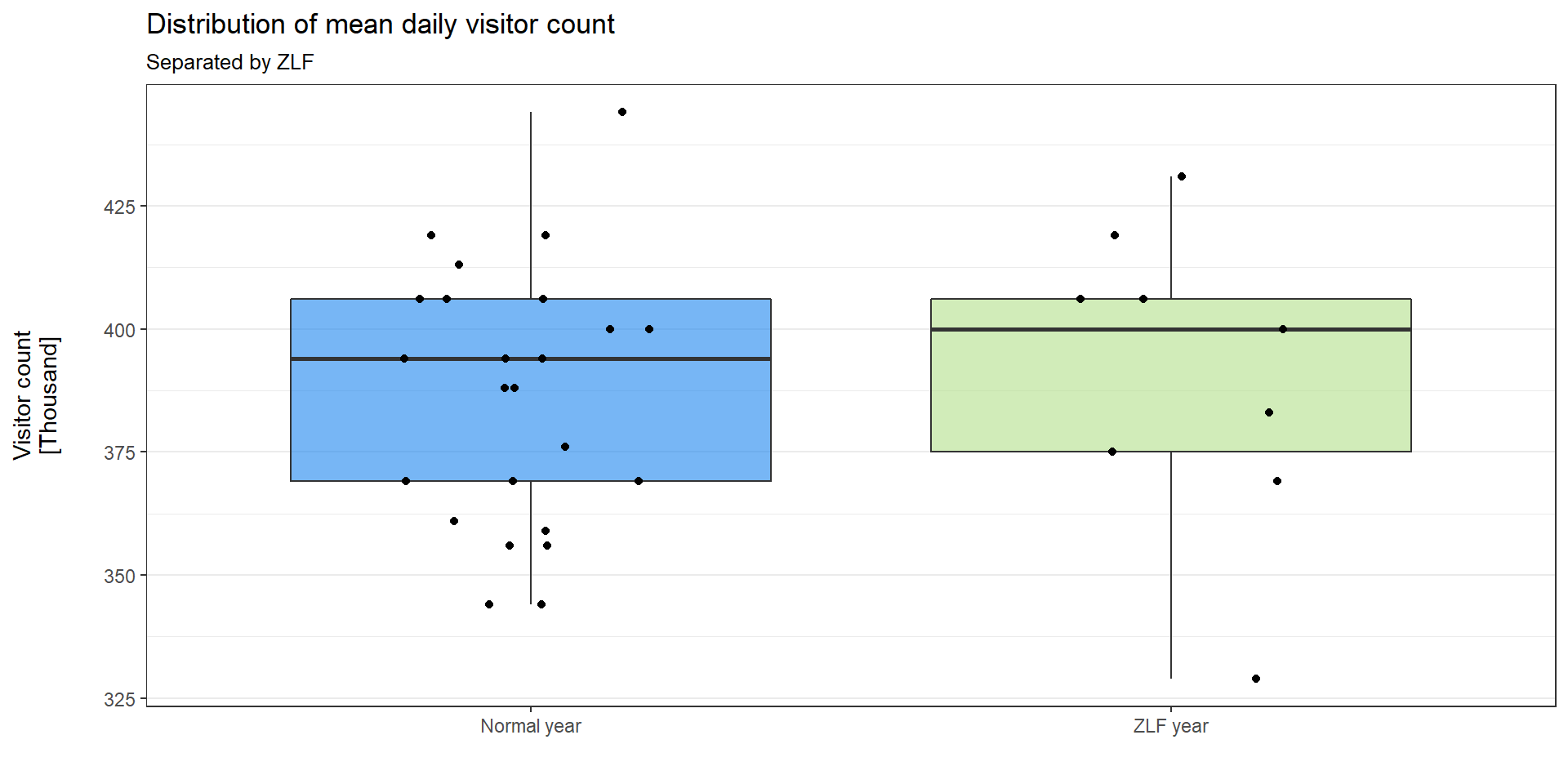
It looks like both box plots are quiet similar. The median of ZLF years is sligthly higher. Nevertheless, we need to be careful, as we have fewer data points for ZLF years than we do for normal years.
We will continue with testing the null hypothesis:
“ZLF years do not have an impact on mean daily visitor count”
To do so we first start with a test for normal distribution in order to select a proper statistical test for comparison. We are going to use the Shapiro-Wilk test for that purpose. It tests the null hypothesis that the data is normally distributed.
# test for normal distribution of ZLF years
shapiro.test(dt[dt$zlf == 1,]$visitors_day)
##
## Shapiro-Wilk normality test
##
## data: dt[dt$zlf == 1, ]$visitors_day
## W = 0.9461, p-value = 0.6473# test for normal distribution of normal years
shapiro.test(dt[dt$zlf == 0,]$visitors_day)##
## Shapiro-Wilk normality test
##
## data: dt[dt$zlf == 0, ]$visitors_day
## W = 0.96318, p-value = 0.4814The outcome of the Shapiro-Wilk test suggests that both groups have normal distributed values. The quantile-quantile plot also supports this, except of a few outliers at the ends:
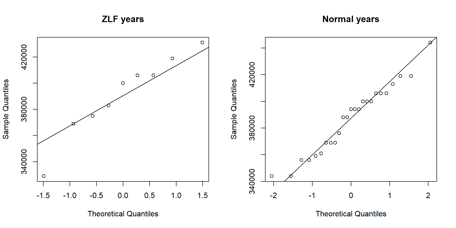
We will assume that our data is normally distributed and continue with a t-test to compare the means of the two groups:
t.test(visitors_total ~ zlf, data = dt)##
## Welch Two Sample t-test
##
## data: visitors_total by zlf
## t = -0.50553, df = 12.282, p-value = 0.6221
## alternative hypothesis: true difference in means is not equal to 0
## 95 percent confidence interval:
## -454537.6 282982.0
## sample estimates:
## mean in group 0 mean in group 1
## 6292000 6377778The outcome of our tests confirms the null hypothesis (the difference in means is equal to 0).
This means that, given this results, the mean daily Oktoberfest visitor count in ZLF years is not statistically different to normal years
Did the Visitors Consume More Beer in ZLF Years?
Now that we know that the ZLF did not bring more visitors to the Oktoberfest, we could ask whether the visitors consumed more beer in ZLF years. We are going to take a part of the beer consumption plot from part 1 and color the ZLF years:
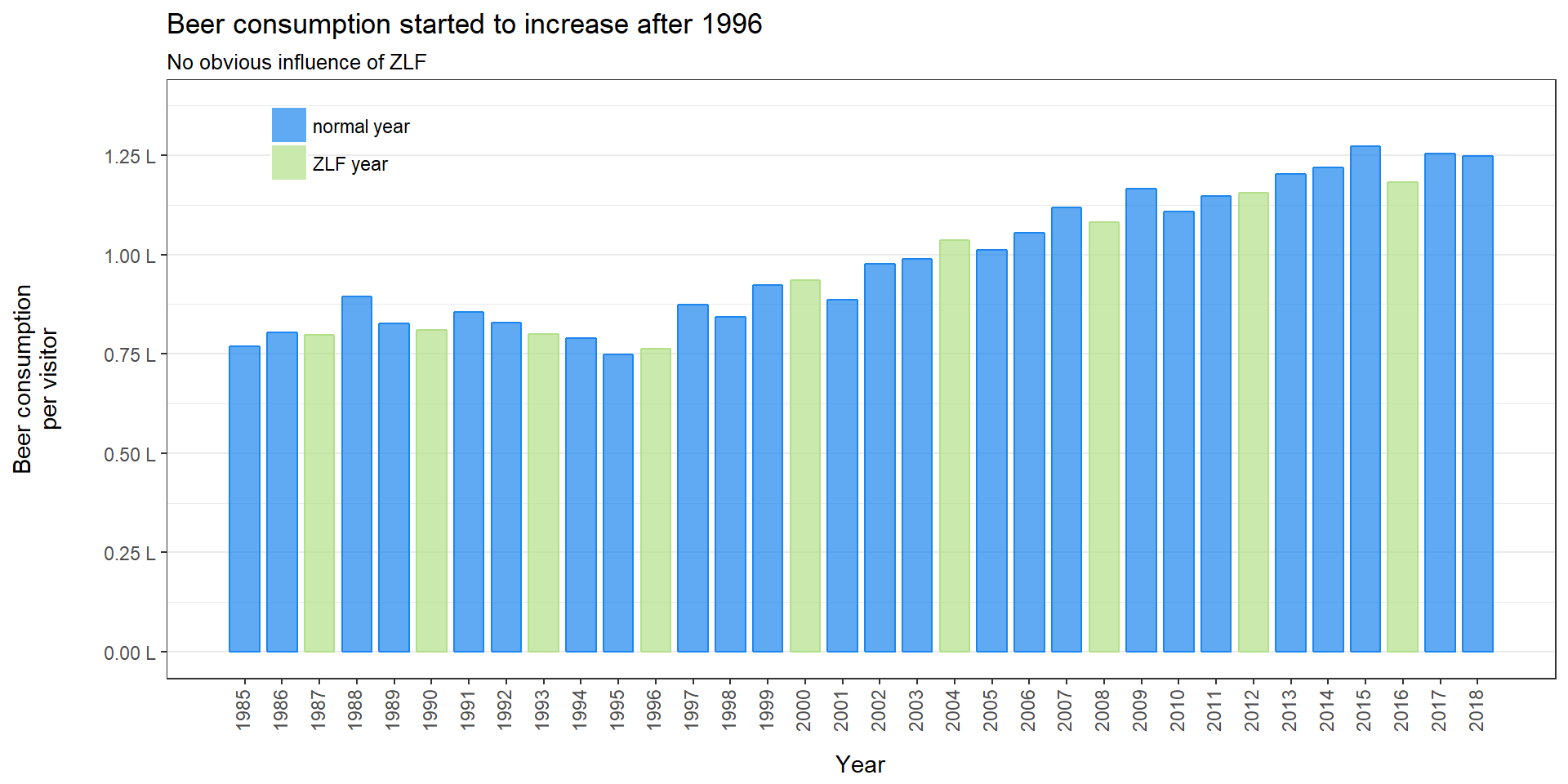
At a first view we cannot see any differences in years with and years without the ZLF. They both follow a similar development. We are going to use the same procedure as above to test for differences. But first a look at the box plots:
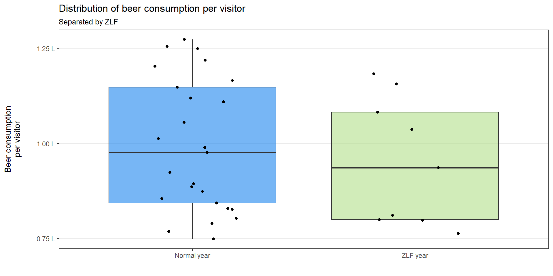
Both box plots look similar again but the ZLF year data seems to be split. We now start with a test for normal distribution and continue with a proper statistical comparison test:
# test for normal distribution of ZLF years
shapiro.test(dt[dt$zlf == 1,]$beer_cons_per_visitor)
##
## Shapiro-Wilk normality test
##
## data: dt[dt$zlf == 1, ]$beer_cons_per_visitor
## W = 0.87501, p-value = 0.139# test for normal distribution of normal years
shapiro.test(dt[dt$zlf == 0,]$beer_cons_per_visitor)##
## Shapiro-Wilk normality test
##
## data: dt[dt$zlf == 0, ]$beer_cons_per_visitor
## W = 0.91753, p-value = 0.04502The outcome of the Shapiro-Wilk test again suggests that both groups have normal distributed values. Nevertheless the p-value is way smaller than before.
The quantile-quantile plot shows us why: The lower and higher quantiles don’t fit the line well.
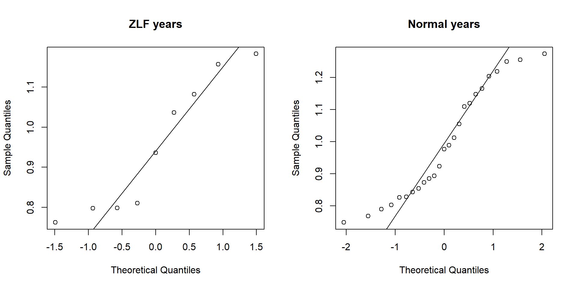
We could again assume a normal distribution, but in my opinion we should try a non-parametric test
here. We are going to use the Mann-Whitney-U-test to compare the groups. In R this test can be performed
using the wilcox.test() function.
wilcox.test(beer_cons_per_visitor ~ zlf, data = dt, conf.int = T)##
## Wilcoxon rank sum test
##
## data: beer_cons_per_visitor by zlf
## W = 132, p-value = 0.4652
## alternative hypothesis: true location shift is not equal to 0
## 95 percent confidence interval:
## -0.1009945 0.1783459
## sample estimates:
## difference in location
## 0.04383077The test result suggests that there is no statistical difference in beer consumption per visitor between ZLF and normal years.
Did the Visitors Consume More Hendl in ZLF Years?
In the last part of our analysis of the ZLF and its influence we are going to look at the hendl consumption. The analysis is going to be performed the same way as above.
Again, we start with a colored plot of the hendl consumption development and two box plots:
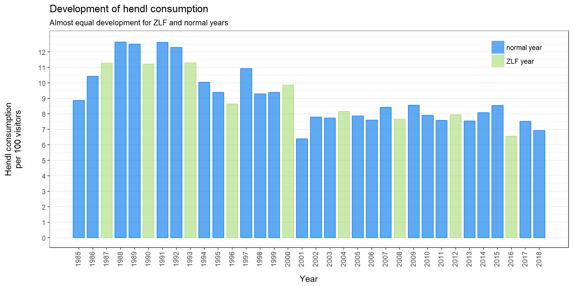
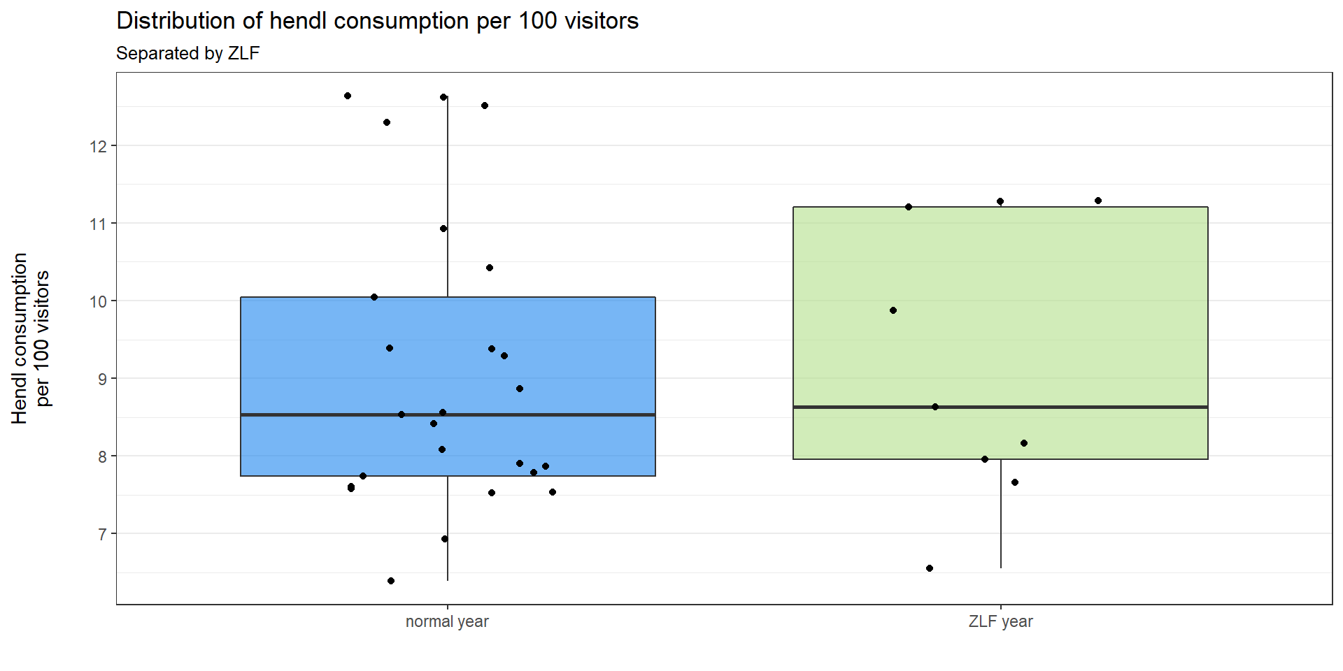
The data distribution looks not very similar for years with and without ZLF. The ZLF boxplot is a little bit more widespread than the other. Nevertheless, we are going to perform our tests as before:
# test for normal distribution of ZLF years
shapiro.test(dt[dt$zlf == 1,]$hendl_cons_per_visitor)
##
## Shapiro-Wilk normality test
##
## data: dt[dt$zlf == 1, ]$hendl_cons_per_visitor
## W = 0.89192, p-value = 0.2088# test for normal distribution of normal years
shapiro.test(dt[dt$zlf == 0,]$hendl_cons_per_visitor)##
## Shapiro-Wilk normality test
##
## data: dt[dt$zlf == 0, ]$hendl_cons_per_visitor
## W = 0.88421, p-value = 0.008449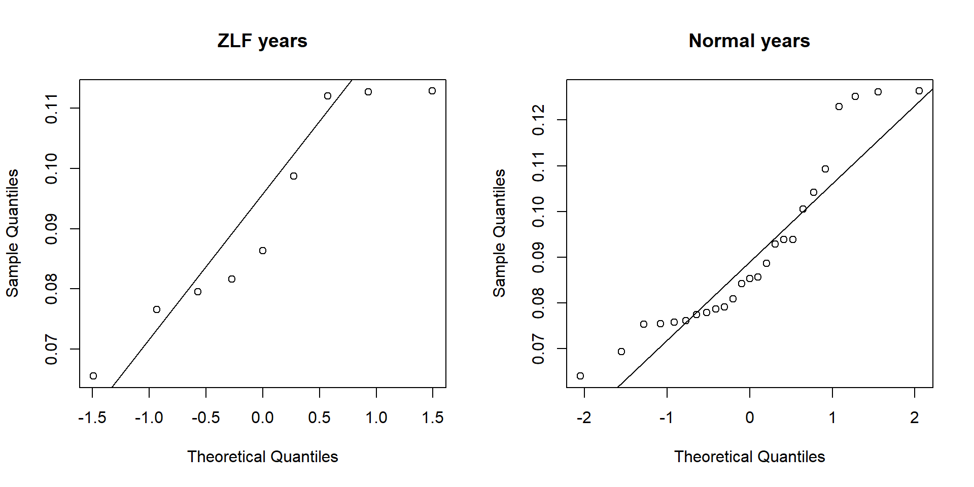
This time the test for normal distribution suggests that at least the normal year data is not normally distributed. That means we definitely need a non parametric test to compare the group means.
wilcox.test(hendl_cons_per_visitor ~ zlf, data = dt, conf.int = T)##
## Wilcoxon rank sum test
##
## data: hendl_cons_per_visitor by zlf
## W = 102, p-value = 0.7014
## alternative hypothesis: true location shift is not equal to 0
## 95 percent confidence interval:
## -0.01888336 0.01236117
## sample estimates:
## difference in location
## -0.001684179The Wilcoxon test confirms our impression that there is no statistical difference between the mean hendl consumption of both groups.
Mean Daily Visitor Count Before and After 9/11
Finally we will look at the hypothesis that the mean daily visitor count decreased to a lower level after the 9/11 terror attacks. During the analysis above we saw a huge drop.
The boxplot below shows the mean daily visitor distribution of both periods:
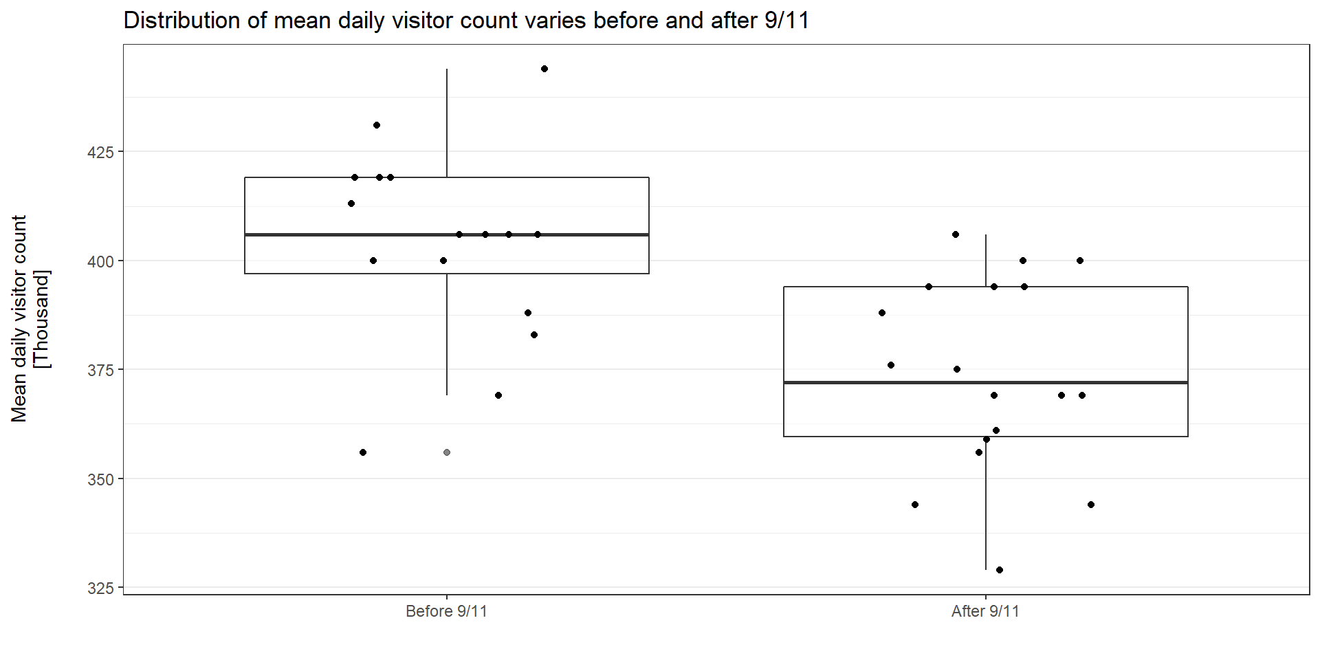
The boxplots show the distribution of mean daily visitor count before and after 9/11 varies. Let’s see what the comparison tests suggest:
# test for normal distribution of data before 2000
shapiro.test(dt[dt$year < 2000,]$visitors_day)
##
## Shapiro-Wilk normality test
##
## data: dt[dt$year < 2000, ]$visitors_day
## W = 0.93676, p-value = 0.3434# test for normal distribution of data after 2000
shapiro.test(dt[dt$year >= 2000,]$visitors_day)##
## Shapiro-Wilk normality test
##
## data: dt[dt$year >= 2000, ]$visitors_day
## W = 0.95688, p-value = 0.5125res <- t.test(visitors_day ~ ifelse(year <= 2000, "After 9/11", "Before 9/11"),
data = dt, conf.int = T)
res##
## Welch Two Sample t-test
##
## data: visitors_day by ifelse(year <= 2000, "After 9/11", "Before 9/11")
## t = 3.9807, df = 31.558, p-value = 0.0003765
## alternative hypothesis: true difference in means is not equal to 0
## 95 percent confidence interval:
## 14806.58 45873.98
## sample estimates:
## mean in group After 9/11 mean in group Before 9/11
## 404062.5 373722.2The t-test confirms our hypothesis. The estimated decrease in daily visitors after 9/11 is 30340 visitors. The 95% confidence interval for the difference is 14806 to 45873 visitors. If we take the mean daily visitor count across the years before 9/11 that would mean a 8 % decrease. Nevertheless, keep in mind that the 9/11 terror attack could just be one reason. There are a lot of other possible reasons which have not been investigated in this analysis.
Conclusion
In the second part of our analysis we showed that…
The years where the ZLF took place did not bring more visitors to the Oktoberfest, nor did it increase the beer or hendl consumption
After the terror attacks in 9/11 the mean daily visitor count decreased by around 8 %.
Update 2019
Added data from 2018
Acknowledgement
For this part I would like to say thank you to the people who helped me with the ressources for that analysis.I would like to thank Frank Börger and the team from Munich Open Data for answering my questions on the data and providing additional resources. Another great thank you goes to my friend Pat forproofreading. Unfortuantely I could not find enough additional visitor data for the ZLF to provide further insights. Nevertheless, I want to thank Mrs Katharina Höninger (Agrarhistorische Bibliothek) and Mrs Christine Karrer (Bayerischer Bauernverband) for their support.
