By Bogdan Oporowski CC BY-SA 3.0, from Wikimedia Commons

San Francisco Crime Heatmaps in R Using BigQuery bigrquery and ggmap

May 27, 2018 11 min read Tutorials

The aim of today’s blog post is to give a short introduction into the usage of BigQuery inside of R. BigQuery is a product within the Google Cloud Platform and serves as a data warehouse for storage and analytics at high scale. It supports standard SQL dialect which makes it easy to use for people with SQL experience.

We are going to use one of the public data sets available on BigQuery and have a short look at the recorded incidents of the San Francisco Police Departments. Further, we are going to plot the data on a map to see areas with high crime densities.

What you are going to learn in this blogpost:

How to use the bigrquery package
How to plot data on a map using the ggmap package
How to use the Google Maps Geocoding API to convert addresses to latitude / longitude data.

Installation and Environment Setup

First things first: There is a package called bigrquery which can be used to query BigQuery tables from R. You can find some quick start information about the bigrquery package on GitHub at https://github.com/r-dbi/bigrquery. The package is also available on CRAN so you can install it using the install.packages() command.

if (!require("bigrquery", quietly = T)) {
  install.packages("bigrquery")
}

We also need to install the newest ggmap version from GitHub, since we need at least version 2.7 to support the Google Maps API for our geocoding of addresses later.

# If you need to install ggmap just uncomment the line below
#devtools::install_github("dkahle/ggmap")

After installing the packages we load them together with the tidyverse package which we are going to use, too.

library("bigrquery", quietly  = T, warn.conflicts = F)
library("tidyverse", quietly  = T, warn.conflicts = F)
library("ggmap", quietly = T, warn.conflicts = F)

Google Cloud Platform Setup

In order to be able to use BigQuery you need to have a Google account. Further, you need to connect your account with Google Cloud Platform (GCP) and create a project there. This is essential for BigQuery because it will need a billing project. All GCP products need to be assigned to a certain project since Google’s billing for the service usage is project based.

Nevertheless, GCP will not charge you for every single service use. There are a lot of services which provide you with some free usage limit per month. Further, if you connect your account with GCP the first time, they give you a free 300$ credit for 12 a months period. You can use this credit for any product on GCP.

The following page will give you access to the free trial and provide you with some additional information about the products and their monthly free usage limits: https://cloud.google.com/free/

After you have created your GCP project, we can start with using BigQuery.

BigQuery and the `bigrquery` Package

As written in the GitHub page README there a basically three possibilities to use the bigrquery package:

The low-level API (BigQuery REST API)
The DBI Interface (for DBI library like interactions)
The dplyr Interface

I am only going to show you the first method but you can read about the others in the README. To get started we need to provide a project-id for billing purpose:

billing <-  project_id # insert your gcp project-id here

This is basically all what we needed to do in order to get everything set up for our work with BigQuery.

Query Examples Using the San Francisco Police Department Data

As mentioned above, we will use a public BigQuery table which provides data of all San Francisco police departments. You can have a look at the table by using the preview function on the BigQuery table page. Google won’t charge you for the previews, but if you press the Query Table button and run SQL queries on the table, you will get charged for each query depending on the data amount it needs to process. But don’t be afraid: The first 1TB each month are for free, so we won’t have a problem running our analysis.

We are going to run 3 queries to ask the following questions on the data:

On which weekday did the most incidents happen?
On which weekday did most arrestments happen and is it the same day as in the first question?
Where do we find the highest crime density within San Francisco? (Here we are going to use ggmap)

Incidents per Weekday

To get the incidents per weekday, we run the following SQL command:

sql <- "
SELECT 
  dayofweek,
  COUNT(*) AS incidents
FROM 
  `bigquery-public-data.san_francisco.sfpd_incidents`
GROUP BY 
  dayofweek
"

We take this SQL command and use the bq_project_query() function from the bigrquery package. It will need a billing project variable for which we use our project-id (the billing variable we created earlier). The function will save our results into a table in BigQuery (either temporary or provided by the user). Then we can use the bq_table_download() function to download our table and use it within R.

bq_dt <- bq_project_query(billing, sql)
dt <- bq_table_download(bq_dt, quiet = TRUE)

Now that we downloaded the data we can also plot it:

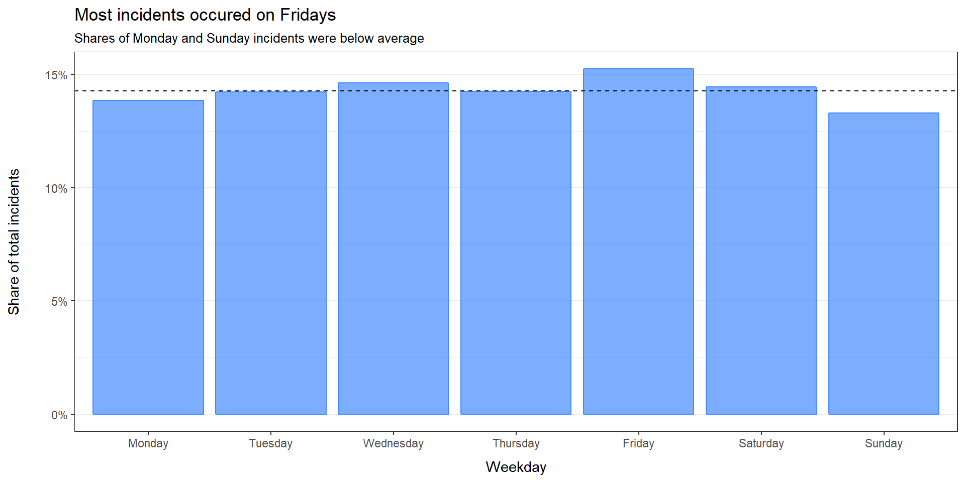
The data show that most incidents happened on Fridays. The proportion of incidents on Fridays was above average, where else the fewest incidents happened on Sundays. Does that really mean that also the worse crime incidents used to happen on Fridays or is this high proportion due to minor crimes committed by people going out? We can use the resolution column and just look for incidents with arrestment. So our next question will be:

On which weekday did most arrestments happen?

Most Arrestings

To answer the question we need to adjust our SQL query from above. We use the bq_project_query() and bq_table_download() command again to get the data.

sql <- '
SELECT 
  dayofweek,
  COUNT(*) AS incidents
FROM 
  `bigquery-public-data.san_francisco.sfpd_incidents`
WHERE 
  resolution LIKE "%ARREST%"
GROUP BY 
  dayofweek
'

bq_dt <- bq_project_query(billing, sql)
dt2 <- bq_table_download(bq_dt, quiet = TRUE)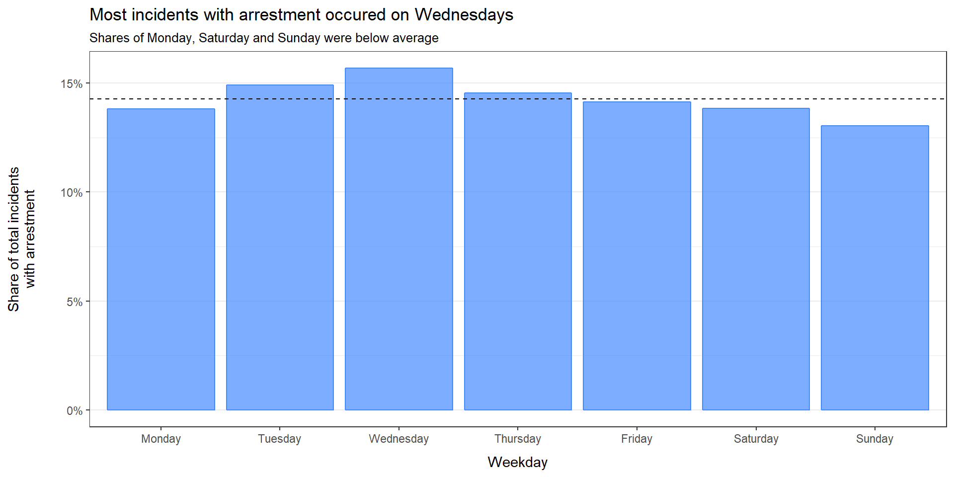

Most of the incidents with arrestment accured on Wednesdays. Although Fridays counted most incidents in the plot before, the proportion for incidents with arrestment on Fridays is just average. Furthermore, it’s interesting that the proportion on other weekdays did not change much.

San Francisco 2017 Crime Map Using the `ggmap` Package

The following information is cited from the Wikipedia article (as of Mai 2018):

“The SFPD currently has 10 main police stations throughout the city in addition to a number of police substations.

Metro Division:

Central Station: 766 Vallejo St. San Francisco, CA 94133
Mission Station: 630 Valencia St. San Francisco, CA 94110
Northern Station: 1125 Fillmore St. San Francisco, CA 94115
Southern Station, Public Safety Building: 1251 3rd St. San Francisco, CA 94103
Tenderloin Station: 301 Eddy St. San Francisco, CA 94102

Golden Gate Division:

Bayview Station: 201 Williams Ave. San Francisco, CA 94124
Ingleside Station: 1 Sgt. John V. Young Ln. San Francisco, CA 94112-2408
Park Station: 1899 Waller Street San Francisco, CA 94117
Richmond Station: 461 6th Ave San Francisco, CA 94118
Taraval Station: 2345 24th Ave. San Francisco, CA 94116"

We are going transform the given addresses into latitude and longitude data to plot them on our heat map later. To do so, we will use the Google Maps Geocoding API with the geocode function of the ggmap package. geocode takes addresses and provides you with latitude / longitude data by querying the Google API (you could also use the Data Science Toolkit as resource). The function can be used with a public API-key but then you might get in trouble with the limits of the public key because it only allows a certain limit of requests.

Since you already created a GCP project, it is easy to get your own API-key for Google Maps Geocoding API. Just visit the developer documentation and follow the instructions. It will tell you how to active the API in your GCP project. After that, Google will provide you with a key which you can use in the code chunk below. I saved my key as a .txt file within this R-Project(./additional_data/api-key.txt).

api_key <- read_lines("./additional_data/api-key.txt") #you would need to insert your api key here

addresses <- c(Central = "766 Vallejo St. San Francisco",
              Mission =  "630 Valencia St. San Francisco",
              Northern = "1125 Fillmore St. San Francisco",
              Southern = "1251 3rd St. San Francisco",
              Tenderloin = "301 Eddy St. San Francisco",
              Bayview = "201 Williams Ave. San Francisco",
              Ingleside = "1 Sgt. John V. Young Ln. San Francisco",
              Park = "1899 Waller Street San Francisco",
              Richmond = "461 6th Ave San Francisco",
              Taraval = "2345 24th Ave. San Francisco")

register_google(api_key)
pd_location <- geocode(addresses, messaging = FALSE)

Let’s check what geocode gave us:

pd_location

##           .id       lon      lat
## 1     Central -122.4100 37.79872
## 2     Mission -122.4220 37.76285
## 3    Northern -122.4325 37.78022
## 4    Southern -122.3894 37.77238
## 5  Tenderloin -122.4130 37.78367
## 6     Bayview -122.3980 37.72976
## 7   Ingleside -122.4463 37.72468
## 8        Park -122.4553 37.76780
## 9    Richmond -122.4645 37.78001
## 10    Taraval -122.4815 37.74371

As you see, it gave us a table with a id (name of our police department) and the corresponding lat / lon data. We ware going to use this data to add the police departments to our map later.

Getting Crime Incidents and their Location

To get the crime data for our map we make another query on the san_francisco.sfpd_incidents table:

sql <- "
SELECT 
  location,
  timestamp,
  dayofweek

FROM 
  `bigquery-public-data.san_francisco.sfpd_incidents`
"
bq_dt <- bq_project_query(billing, sql)
dt4 <- bq_table_download(bq_dt, quiet = TRUE)

We now need extract latitude / longitude data from the location column and filter it since there is a outlier in the data.

dt4 <- dt4 %>% 
  mutate(location = gsub("\\(|\\)| ","",location)) %>% 
  separate(location, sep = ",", into = c("lat","long")) %>% 
  mutate(lon = as.numeric(long),
         lat = as.numeric(lat),
         year = format(timestamp, "%Y")) %>% 
  filter(lat < 90)

Now we can get our hands dirty and start creating the heat map plot.

Creating the Heatmap for 2017

What we need to do first is creating a area-box for our map. This can be done using the make_bbox() function. This area can be used to download a plot map using the get_map() function.

area <- make_bbox(lon = lon, lat = lat, data = dt4)
area

##       left     bottom      right        top 
## -122.52109   37.70224 -122.35731   37.82626

area_map <- get_map(area,  source = "stamen")
ggmap(area_map, extend = "device", darken = 0.2)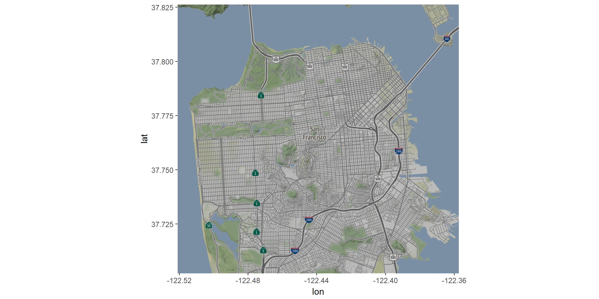

Perfect! We got our map and used the ggmap() function to plot it. Now we can just add ggplot layers as known from ggplot. In our example we use the stat_density2d() layer to create a heat map with 2017s data. We will also add labels for the position of the Police Departments:

ggmap(area_map, extend = "device", darken = 0.3) +
  stat_density2d(aes(x = lon, y = lat, fill = ..level../10), alpha = 0.2,
                 data = subset(dt4, year == "2017"), geom = "polygon", bins = 30) +
  geom_label(aes(x = lon, y = lat, label = .id), data = pd_location, size = 3, alpha = 0.5) +
  scale_fill_gradient2(low = "yellow", mid = "orange", high = "firebrick2", midpoint = 80,
                       guide = guide_colorbar(title = "Level")) +
  geom_text(aes(x = -122.41, y = 37.82, label = "San Francisco Crimes 2017"), size = 6,
            color = "white") +
  theme_void() +
  theme(legend.position = c(0.15,0.93),
        legend.direction = "horizontal",
        legend.background = element_rect(fill = alpha("white", 0.8), 
                                  size = 0.5, linetype = "solid"))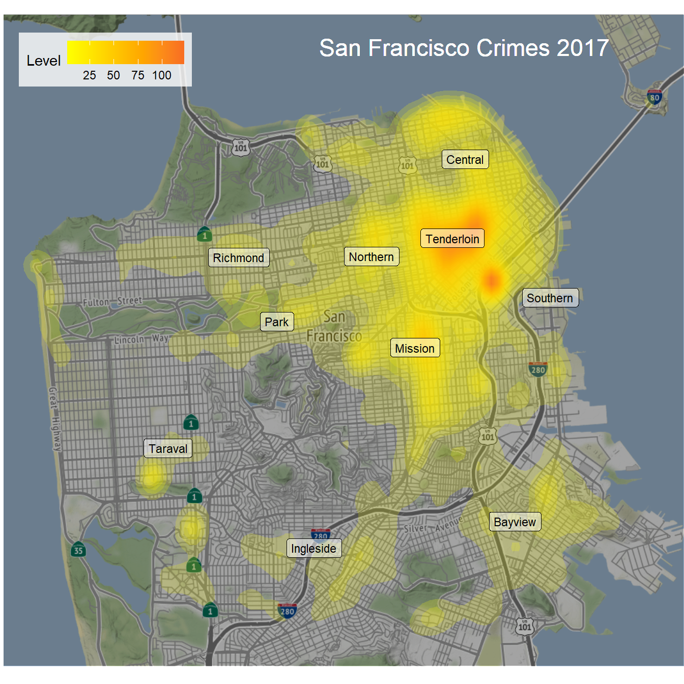

Another possibility would be to use geom_point() to plot every single crime instance and use the alpha parameter to adjust for a correct density representation:

ggmap(area_map, extend = "device", darken = 0.3) +
  geom_point(aes(x = lon, y = lat), alpha = 0.02, size = 1.5, color = "orange",
                 data = subset(dt4, year == "2017")) +
  geom_label(aes(x = lon, y = lat, label = .id), data = pd_location, size = 3, alpha = 0.7) +
  theme_nothing() +
  geom_text(aes(x = -122.41, y = 37.82, label = "San Francisco Crimes 2017"), size = 6,
            color = "white") +
  theme(legend.position = c(0.2,0.93),
        legend.direction = "horizontal",
        legend.background = element_rect(fill = alpha("white", 0.8), 
                                  size = 0.5, linetype = "solid"))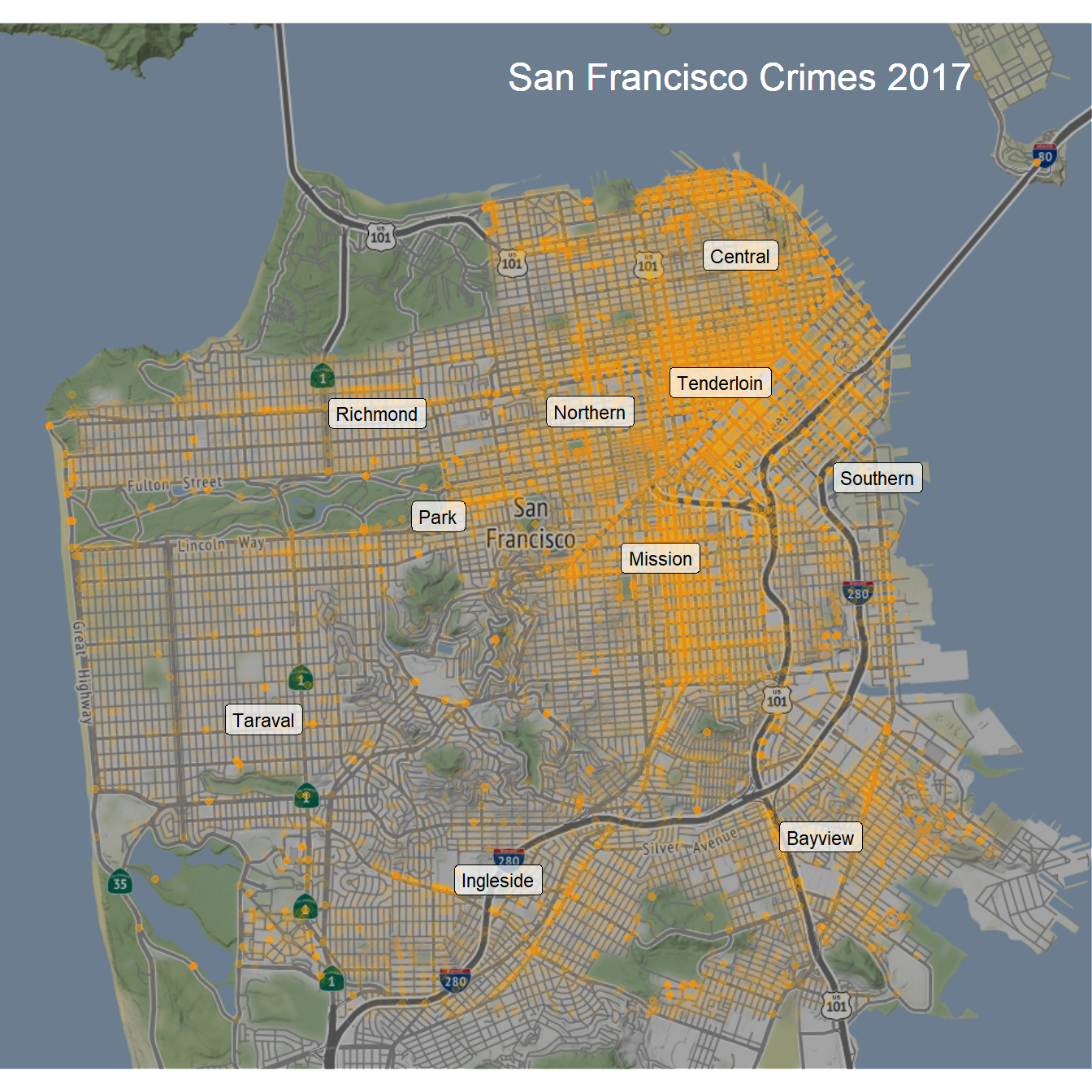

As we see, there have been a lot of incidents around Tenderloin and Southern district. You better be careful when visiting that area.

Conclusion and Further Ressources

We went through a short introduction into bigrquery and the ggmap package. We learned how to query data from BigQuery and how to plot that data on a map. Further, we used the Google Maps Geocoding API to transform addresses into latitude and longitude data.

At this point I want to provide a summary of useful ressources:

BigQuery:

Google Cloud Platform getting started page to create your first GCP project
Official Big Query page for information about the product as well as documentation
BigQuery sample tables which you can use to play around with
BigQuery web user interface where you can make some queries after having created a project
Bigrquery GitHub page for documentation and further usage examples

Google Maps Geocoding API:

GCP API Library where you can activate the Geocoding API withing GCP
Geocoding Documentation - get a key - here you can follow the steps to request your personal API key

ggmap Package:

ggmap Github page - here you find more detailed information on the usage of ggmap and the geocode() function

Thank you for reading this blog post. As always: If you have any questions, corrections, interesting additional information or just want to add something else, feel free to comment or contact me.

R BigQuery bigrquery ggmap geocoding